In [161]:
image = Image.open('habitat_67_small.jpg').convert("L")
img_mat = np.asarray(image)
fig = plt.imshow(img_mat, cmap='gray')
fig.axes.get_xaxis().set_visible(False)
fig.axes.get_yaxis().set_visible(False)

Using SVD (Singular Value Decomposition), we can achieve a basic form of image compression. In this case, we can represent an image as a matrix of grayscale values (ranging from 0 to 255) and compute the SVD, resulting in $\text{US}{V}^{T}$. To compress the image to a smaller size, we will preserve the first $\text{k}$ singular values found in $\text{S}$, the first $\text{k}$ columns of $\text{U}$ and the first $\text{k}$ rows of $\text{V}^{T}$ and multiply the three components back together. The singular values are ordered in importance to the image's quality, meaning that the lower our $\text{k}$ is, the worse our quality will be.
import math; import PIL; from PIL import Image; import numpy as np; import matplotlib.pyplot as plt
Here's our original image:
image = Image.open('habitat_67_small.jpg').convert("L")
img_mat = np.asarray(image)
fig = plt.imshow(img_mat, cmap='gray')
fig.axes.get_xaxis().set_visible(False)
fig.axes.get_yaxis().set_visible(False)
Now, with compression preserving the first 30 and 10 singular values, from left to right.
U, s, V = np.linalg.svd(img_mat, full_matrices=True)
s = np.diag(s)

plt.figure(figsize=(15, 10), dpi=40)

plt.subplot(1,2,1)

k = 30
compressed_by_k = U[:, :k] @ s[0:k, :k] @ V[:k, :]

fig = plt.imshow(compressed_by_k, cmap='gray')
fig.axes.get_xaxis().set_visible(False)
fig.axes.get_yaxis().set_visible(False)

plt.subplot(1,2,2)

k = 10
compressed_by_k = U[:, :k] @ s[0:k, :k] @ V[:k, :]

fig = plt.imshow(compressed_by_k, cmap='gray'); fig.axes.get_xaxis().set_visible(False); fig.axes.get_yaxis().set_visible(False); plt.show()

The JPEG image compression algorithm consists of a series of transformations - only one of which is non-reversable. This non-reversable transformation is what makes this compression "lossy"
The crux of DCT, and thus the key to JPEG compression, is the fact that every 8x8px 2-color image can be represented as a weighted linear combination of basis images given by cosine waves
$\text{imagePixel}_{i,j} = \sum_{u=0}^{7} \sum_{v=0}^{7} a_{u,v} \cos{(\frac{\pi u (2i+1)}{16})}\cos{(\frac{\pi v (2j+1)}{16})}$ Where $a_{u,v}$ is some coefficient
Below is a visualization of each of the 64 basis images (functions) for an 8x8px image (shown for black and white) given by the equation:
$\text{basisPixel}_{u,v,i,j} = \cos{(\frac{\pi u (2i+1)}{16})}\cos{(\frac{\pi v (2j+1)}{16})}$ where i,j is the index of each pixel for the given basis image u,v.
def print_image(array, colors):
    fig = plt.imshow(array); fig.set_cmap(colors); fig.axes.get_xaxis().set_visible(False); fig.axes.get_yaxis().set_visible(False); plt.show()

output=np.zeros((73,73), dtype=np.float16)
for u in range(0,8):
    for v in range(0,8):
        for i in range(0,8):
            for j in range(0,8):
                output[(9*u)+i+1][(9*v)+j+1] = math.cos(math.pi*u*(2*i+1)*(1/16)) * math.cos(math.pi*v*(2*j+1)*(1/16)) * 127 + 127
print_image(output, 'Greys')

There are basis images for any dimensions of the image, but JPEG looks at 8x8 chunks because the number of basis images is equivalent to the number of pixels in an image, but adding just one extra pixel to the width adds height new basis images, so it is important to strike a balance between the size of the chunks and the number of basis images.
The discrete cosine transform is a process by which a matrix, in this case a matrix of pixel brightness values, is decomposed (similar to singular value decomposition) to find the weights of each basis image.
$\text{BasisWeight}_{u,v} = \frac{1}{4} \sum_{i=0}^{7} \sum_{j=0}^{7} C(u) C(v) \cos{(\frac{\pi u (2i+1)}{16})}\cos{(\frac{\pi v (2j+1)}{16})} \text{ImagePixels}_{i,j}$
The C(x) function is compensating for the fact that if u or v is 0, one of the cos functions becomes a constant value of 1.
$C(x) = \begin{cases} \frac{\sqrt{2}}{2} &\quad\text{if } x=0\\ 1 &\quad\text{otherwise} \\ \end{cases}$
Because this transformation is lossless, we can restore the original image by using a similar equation.
$\text{ImagePixels}_{i,j} = \frac{1}{4} \sum_{u=0}^{7} \sum_{v=0}^{7} C(u) C(v) \cos{(\frac{\pi u (2i+1)}{16})}\cos{(\frac{\pi v (2j+1)}{16})} \text{BasisWeight}_{i,j}$
The code below defines the DCT and reverse DCT function for an 8x8 matrix.
class DCT:

   # scale for inside the sum
   def C(self,i,j):
      if (i==0 and j==0):
         return 1/2
      elif (i==0 or j==0):
         return 1/math.sqrt(2)
      else:
         return 1

   # Forward DCT (8x8)
   def DCT(self, image_pixels):
      basis_weights=np.zeros((8,8), dtype=np.int16)
      cos_sum=0

      for u in range(0,8):
         for v in range(0,8):
            for i in range(0,8):
               for j in range(0,8):
                  cos_sum += self.C(u,v) * math.cos(math.pi*u*(2*i+1)*(1/16)) * math.cos(math.pi*v*(2*j+1)*(1/16)) * image_pixels[i][j]
            basis_weights[u][v] = (1/4)*cos_sum
            cos_sum = 0

      return basis_weights

   # Inverse DCT
   def IDCT(self, basis_weights):
      image_pixels=np.zeros((8,8), dtype=np.int16)
      cos_sum=0

      for i in range(0,8):
         for j in range(0,8):
            for u in range(0,8):
               for v in range(0,8):
                  cos_sum += self.C(u,v) * math.cos(math.pi*u*(2*i+1)*(1/16)) * math.cos(math.pi*v*(2*j+1)*(1/16)) * basis_weights[u][v]

            image_pixels[i][j] = int(round((1/4)*cos_sum, 0))
            cos_sum = 0

      return image_pixels
dct = DCT()
image = np.array([[1+x,2+x,3+x,4+x,5+x,6+x,7+x,8+x] for x in range(0,8)])
coefficients = dct.DCT(image)
new_image = dct.IDCT(coefficients)

print("Original Image:")
print_image(image, 'Greys')
print("Basis weights:")
print(coefficients)
Original Image:

Basis weights:
[[ 64 -18   0  -1   0   0   0   0]
 [-18   0   0   0   0   0   0   0]
 [  0   0   0   0   0   0   0   0]
 [ -1   0   0   0   0   0   0   0]
 [  0   0   0   0   0   0   0   0]
 [  0   0   0   0   0   0   0   0]
 [  0   0   0   0   0   0   0   0]
 [  0   0   0   0   0   0   0   0]]
But if we always have the same number of basis image weights as pixels in the image, how will we save any storage space? This is where quantization is helpful. The process of quantization eliminates basis images that the human eye would have a difficult time differentiating. This is similar to eliminating the lowest values from the $\Sigma$ matrix produced through SVD.
We employ a quantization table - an 8x8 matrix of values fine-tuned to specifically reduce less-noticable weights. The values in the table determine how heavily the image is compressed. JPEG uses two different tables - one for the luminance, and a second more aggressive table for the two chrominance channels (it is easier to notice inconsistencies in brightness than color). This contributes to JPEG artifacts on edges of objects, as the more compressed color channels do not perfectly overlap the brightness channel.
To quantize a basis weight: $\text{QuantizedValue}_{u,v} = \lceil\frac{\text{BasisWeight}_{u,v}}{\text{QuantizationTable}_{u,v}}\rfloor$
This has the effect of reducing large weights for storage, while rounding off weights of lesser importance. If a weight is less than its value in the table, it becomes 0, which becomes useful later on. This rounding is the irreversable lossy operation which makes JPEG a lossy compression. When the weights are restored to reconstruct the image, some of the basis images are dropped due to rounding error.
The following class calculates quantization and inverse quantization:
class Qunatization:
    def __init__(self):
        self.LUMINANCE_TABLE = np.array([[16, 11, 10, 16, 24, 40, 51, 61],[12, 12, 14, 19, 26, 58, 60, 55],[14, 13, 16, 24, 40, 57, 69, 56],[14, 17, 22, 29, 51, 87, 80, 62],[18, 22, 37, 56, 68, 109, 103, 77],[24, 35, 55, 64, 81, 104, 113, 92],[49, 64, 78, 87, 103, 121, 120, 101],[72, 92, 95, 98, 112, 100, 103, 99]])
        self.CHROMINANCE_TABLE = np.array([[17, 18, 24, 47, 99, 99, 99, 99], [18, 21, 26, 66, 99, 99, 99, 99], [24, 26, 56, 99, 99, 99, 99, 99], [47, 66, 99, 99, 99, 99, 99, 99], [99, 99, 99, 99, 99, 99, 99, 99],[99, 99, 99, 99, 99, 99, 99, 99],[99, 99, 99, 99, 99, 99, 99, 99],[99, 99, 99, 99, 99, 99, 99, 99]])

    def quantize(self, basis_weight, table):
        quantized_value = np.zeros((8,8), dtype=np.int16)
        for i in range(0,7):
            for j in range(0,7):
                quantized_value[i][j] = round(basis_weight[i][j]/table[i][j], 0)
        return quantized_value

    def unquantize(self, quantized_value, table):
        basis_weight = np.zeros((8,8), dtype=np.int16)
        for i in range(0,7):
            for j in range(0,7):
                basis_weight[i][j] = quantized_value[i][j] * table[i][j]
        return basis_weight
quantizer = Qunatization()
quantized_values = quantizer.quantize(coefficients, quantizer.LUMINANCE_TABLE)
restored_weights = quantizer.unquantize(quantized_values, quantizer.LUMINANCE_TABLE)
restored_image = dct.IDCT(restored_weights)
print("Original Image:")
print_image(image, "Greys")
print("Compressed Image:")
print_image(restored_image, "Greys")
Original Image:
Compressed Image:

The quantization eliminated some of the fine detail in the image, but at the same time has successfully eliminated some data from the image. it is unlikely that a person would notice this difference, considering that this 8x8px chunk would constitude a tiny part of the full image. Imagine that this the the corner of the letter S below on your computer screen... good luck seeing a difference!
The image is now lossy, meaning it has lost some of its original data. However, it can still be compressed further.
The quantization leaves us with an array consisting of mostly zeros. Because the less noticable basis images are concentrated toward the bottom left of the matrix, the majority of the zeros will be there too. We want to save this matrix in such a way that groups as many zeros together as possible, which is helpful in a later step. The best way to do this is to serialize the matrix as diagonal slices starting in the top left corner and moving toward the bottom right corner. The following class does this to turn the quantized values into an array.
class Encoder:
   def entropy_encode(self, mask):
      output = np.zeros(64, dtype=np.int16)
      output[0] = mask[0][0]; i=0; j=1; level=1; loc=1
      while True:
         # level is even, so we are iterating from left to right
         if (level%2==0):
            if (i<8 and j<8):
               output[loc] = mask[i][j]; loc+=1
            i-=1; j+=1
            # move to the next level
            if (i==-1):
               level+=1; i=0; j=level
         # level is odd, so we are iterating from right to left
         else:
            if (i<8 and j<8):
               output[loc] = mask[i][j]; loc+=1
            i+=1; j-=1
            # move to the next level
            if (j==-1):
               level+=1; j=0; i=level
         if (i==7 and j==7):
            output[loc] = mask[i][j]; return output

   def entropy_decode(self, array):
      output = np.zeros((8,8), dtype=np.int16)
      output[0][0] = array[0]; i=0; j=1; level=1; loc=1
      while True:
         # level is even, so we are iterating from left to right
         if (level%2==0):
            if (i<8 and j<8):
               output[i][j] = array[loc]; loc+=1
            i-=1; j+=1
            # move to the next level
            if (i==-1):
               level+=1; i=0; j=level
         # level is odd, so we are iterating from right to left
         else:
            if (i<8 and j<8):
               output[i][j] = array[loc]; loc+=1
            i+=1; j-=1
            if (j==-1):
               level+=1; j=0; i=level
         if (i==7 and j==7):
            output[i][j] = array[loc]; return output
Encoding the quantized values:
encoder=Encoder()
encoded = encoder.entropy_encode(quantized_values)
print("Quantized values:"); print(quantized_values); print()
print("Encoded values in array:"); print(encoded)
Quantized values:
[[ 4 -2  0  0  0  0  0  0]
 [-2  0  0  0  0  0  0  0]
 [ 0  0  0  0  0  0  0  0]
 [ 0  0  0  0  0  0  0  0]
 [ 0  0  0  0  0  0  0  0]
 [ 0  0  0  0  0  0  0  0]
 [ 0  0  0  0  0  0  0  0]
 [ 0  0  0  0  0  0  0  0]]

Encoded values in array:
[ 4 -2 -2  0  0  0  0  0  0  0  0  0  0  0  0  0  0  0  0  0  0  0  0  0
  0  0  0  0  0  0  0  0  0  0  0  0  0  0  0  0  0  0  0  0  0  0  0  0
  0  0  0  0  0  0  0  0  0  0  0  0  0  0  0  0]
The final step before saving the bytes of the encoded array is a process know as Huffman Coding.
Huffman Coding is the process by which objects are assigned bit representations based on their frequency. If a value appears more frequently than another, the coding algorithm will find a bit representation which contains fewer bits in the whole file as compared to if they had the same representation length. This leverages the computer science data structure known as a binary tree, and can be assembled quite simply. We can look at the basic example of our running example of encoded values, but the algorithm is extensible to an arbitrarily large set of different values.
A vertex in the binary tree (which is a restricted graph) is represented with $\text{V}_{\text{value}}(\text{weight})$. For example, $\text{V}_{4}(1)$ is a vertex with value 4 and weight 1.
Step 1: Count the number of each value in the set and represent each value with its respective count as a vertex weight.
$\lbrace\text{V}_{4}(1), \text{V}_{-2}(2), \text{V}_{0}(61)\rbrace$
Step 2: Assemble the binary tree by combining the two smallest weighted nodes and to a new node of the two weights combined.
$\text{V}_{4}(1) + \text{V}_{-2}(2) = \text{V}_{\lbrace\text{V}_{4}, \text{V}_{-2}\rbrace}(3)$
Add this new vertex back to the list of existing verticies.
$\lbrace\text{V}_{0}(61), \text{V}_{\lbrace\text{V}_{4}, \text{V}_{-2}\rbrace}(3)\rbrace$
This is repeated until there is only one vertex remaining in the to-do list
$\text{V}_{\lbrace\text{V}_{0}, \text{V}_{\lbrace\text{V}_{4}, \text{V}_{-2}\rbrace}\rbrace}(64)$
Step 3: For each vertex, label the branch with a binary 0 for each left branch and 1 on each right branch.
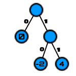
Step 4: Save the data by traversing the tree moving toward the target value and using the bit values on each edge as the code.
To encode the first 5 values in the encoded array, [4, -2, -2, 0, 0] becomes 11 10 10 0 0, turning an (at minimum) 5 byte array into just one single byte. Notice that the vertices with values only appear with no exiting edges, also known as leaf nodes. This makes it possible to load the data again by reversing the process, sequentially reading each bit and moving down the matching edge of the current vertex until arriving at a leaf node. This is the next value. Repeat this until out of bits, and the original array is recovered.
The Huffman Coding algorithm is especially effective for our encoded array, because it contains almost entirely 0s. It can represent each 0 as a single 0 bit, which is smaller than the minimal integer representation by a factor of 8. Here is the Huffman coding executed by the dahuffman library on the full array of 64 8-bit integers. Note that it picks slightly different codes than we did for each vales and must encode an EOF (end of file) code to know when to stop reading from the file (Usually the actual tree and other metadata would be placed after this EOF for other computers to use when decoding).
from dahuffman import HuffmanCodec
codec = HuffmanCodec.from_data(encoded)
codec.print_code_table()
bytes = codec.encode(encoded)
print("Number of bytes before Huffman Coding: " + str(len(encoded)))
print("Number of bytes after Huffman Coding: " + str(len(bytes)))
print("And in bytes, the final image looks like: " + str(bytes))
Bits Code Value Symbol
   3 000      0 _EOF
   3 001      1 4
   2 01       1 -2
   1 1        1 0
Number of bytes before Huffman Coding: 64
Number of bytes after Huffman Coding: 9
And in bytes, the final image looks like: b'+\xff\xff\xff\xff\xff\xff\xff\xf0'
Now it is time to put all of these clever algorithms together in order to compress a real image. We'll perform DCT compression on the same image we performed SVD compression on and see how it holds up.
image = Image.open('habitat_67_small.jpg')

fig = plt.imshow(image)
fig.axes.get_xaxis().set_visible(False)
fig.axes.get_yaxis().set_visible(False)
plt.show()

This time, we'll modify the previously described quantization table based on the desired quality of the image. We'll let the base quantization table $\text{Q}$ have a parameter $\text{quality}$ of $\text{50}$. This parameter can range from $\text{1}$ to $\text{100}$. $\text{Q}$ is multiplied by $\frac{100-quality}{50}$ when $\text{Q}>{50}$ and $\frac{50}{quality}$ when $\text{Q}<{50}$.
h = 256
w = 256
N = 8 #8x8 chunks

dct = DCT()
quantizer = Qunatization()
encoder = Encoder()

def gen_quant_quality(Q, quality):
    if quality>50:
        Q = (Q * ((100-quality)/50)).astype('int')
        Q = np.where(Q>255,255,Q)
    elif quality<50:
        Q = (Q * (50/quality)).astype('int')
        Q = np.where(Q>255,255,Q)
    return Q

def compressChannel(channel, quality, color_channel):
    new_Q = gen_quant_quality(quantizer.CHROMINANCE_TABLE, quality) if color_channel else gen_quant_quality(quantizer.LUMINANCE_TABLE, quality) # selecting correct table

    out = np.zeros(shape=(h*w), dtype=np.int16)
    final_idx = 0;
    for i in range(0,h,N):
        print("Compressing: "+str(100*i/h)+"%      ", end = "\r")
        for j in range(0,w,N):
            entropy_encode = encoder.entropy_encode(quantizer.quantize(dct.DCT(channel[i:i+N, j:j+N]), new_Q))
            for batch_idx in range(0,64):
                out[final_idx] = entropy_encode[batch_idx]
                final_idx+=1
    print("Finished                 ", end = "\r"); return out

def uncompressChannel(compressed_channel, quality, color_channel):
    new_Q = gen_quant_quality(quantizer.CHROMINANCE_TABLE, quality) if color_channel else gen_quant_quality(quantizer.LUMINANCE_TABLE, quality) # selecting correct table
    out = np.zeros(shape=(h,w), dtype=np.int16)
    chunk_num=0

    for i in range(0,h,N):
        print("Uncompressing: "+str(100*i/h)+"%     ", end = "\r")
        for j in range(0,w,N):
            inv_dct = dct.IDCT(quantizer.unquantize(encoder.entropy_decode(compressed_channel[64*chunk_num:64+(64*chunk_num)]), new_Q)) # restoring from encoded array by chunk
            x_counter = 0 # Stitching image back together from chunks
            for x in range(i,i+N):
                y_counter = 0
                for y in range(j,j+N):
                    out[x][y] = inv_dct[x_counter][y_counter]
                    y_counter += 1
                x_counter += 1

            chunk_num+=1
    print("Finished               ", end = "\r")
    return out

plt.figure(figsize=(15, 10), dpi=40)
subplot_counter = 1
byteSize = []
for quality_val in [90, 50, 10, 5]:
    ycbcr = image.convert('YCbCr')
    (Y, Cb, Cr) = ycbcr.split()
    Y, Cb, Cr = np.array(Y).astype(np.int16), np.array(Cb).astype(np.int16), np.array(Cr).astype(np.int16)
    Y, Cb, Cr = Y - 128, Cb - 128, Cr - 128
    Y, Cb, Cr = compressChannel(Y,quality_val, False), compressChannel(Cb,quality_val, True), compressChannel(Cr,quality_val, True)

    encoded_vals = np.concatenate((Y, Cb, Cr)) # measuring the byte size of each image - factors in 512 bytes for worst case size of saved huffman tree
    codec = HuffmanCodec.from_data(encoded_vals)
    bytes = codec.encode(encoded_vals)
    byteSize.append(len(bytes)+255)

    Y, Cb, Cr = uncompressChannel(Y,quality_val, False), uncompressChannel(Cb,quality_val, True), uncompressChannel(Cr,quality_val, True)
    Y, Cb, Cr = Y + 128, Cb + 128, Cr + 128
    Y, Cb, Cr = Y.astype('uint8'), Cb.astype('uint8'), Cr.astype('uint8')

    stacked = np.dstack((Y,Cb,Cr))    # Converting from numpy matrix to image
    fromarray = Image.fromarray(stacked, mode="YCbCr")
    compressed = fromarray.convert('RGB')

    plt.subplot(1,4,subplot_counter)
    fig = plt.imshow(compressed)
    fig.axes.get_xaxis().set_visible(False); fig.axes.get_yaxis().set_visible(False); subplot_counter += 1

plt.show()
print("Size in Kilobytes of each compression")
print([size/1000 for size in byteSize])
Finished

Size in Kilobytes of each compression
[52.012, 34.489, 27.402, 25.967]
Above are samples of compression for $\text{quality}={90}, {50}, {10},$ and $\text{5}$ going from left to right, using the full DCT pipeline.
In conclusion, JPEG is a more computationally intensive but less noticable image compression method compared to SVD.
Forward DCT: https://users.cs.cf.ac.uk/Dave.Marshall/Multimedia/node231.html
://www.math.cuhk.edu.hk/~lmlui/dct.pdf
Backward DCT: https://www.csie.ntu.edu.tw/~b89044/home/IPR/2DINVERSE.pdf
https://towardsdatascience.com/image-compression-dct-method-f2bb79419587
https://fairyonice.github.io/2D-DCT.html
Huffman Coding: https://www.geeksforgeeks.org/huffman-coding-greedy-algo-3/